Scikit-Learn Regression of Hammer Throw Distance

Linear Regression

Linear regression is a fundamental statistical method used in machine learning to model the relationship between a dependent variable (often called the target or outcome) and one or more independent variables (often called features or predictors). In our example of hammer throwing we have 2 inputs (velocity and angle), and one output (distance). The regression equation therefore becomes: $d = b_0 + b_1 v + b_2 \alpha$. The goal of linear regression is to find the values of the coefficients ($b_i$) that minimize the difference between the predicted values and the actual values. This difference is measured using a loss function, commonly the  mean squared error (MSE). In this case it is clear that the distance thrown is not a linear function of the input parameters, so it is unlikely that Linear Regression can accurately predict hammer throwing!

import matplotlib.pyplot as plt
import numpy as np
from sklearn.model_selection import train_test_split
from sklearn.linear_model import LinearRegression
from sklearn.metrics import mean_squared_error, mean_absolute_error 
import timeit

X = np.load('data_X.npy')
Y = np.load('data_Y.npy')

start = timeit.default_timer()
X_train, X_test, y_train, y_test = train_test_split(X, Y, test_size=0.3)
model = LinearRegression()
model.fit(X_train, y_train)
print("model coef =", model.coef_)

predictions = model.predict(X_test)
print(f"Mean absolute error={mean_absolute_error(y_test, predictions):.3f}")

stop = timeit.default_timer()
print(f"Runtime = {stop-start:.5f} sec")

#print(X_test.shape)
#print(predictions.shape)
plt.scatter(X_test[:,1], y_test, c='r')
plt.scatter(X_test[:,1], predictions, c='b')
plt.xlabel('Velocity (m/s)')
plt.ylabel('Distance (m)')

model coef = [1.77601689 3.14936738]
Mean absolute error=19.266
Runtime = 0.00232 sec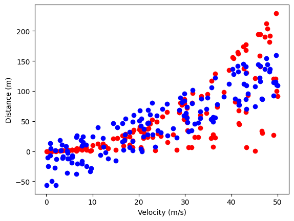

As expected this did not work very well.

Nearest Neighbors Regression

Nearest Neighbors Regression, also known as K-Nearest Neighbors Regression (KNN Regression), is a non-parametric method used for regression tasks in machine learning. KNN Regression predicts the value of a target variable for a new data point by using the values of the target variable for the K-nearest data points in the training set. The prediction is typically the average of the target values of the K-nearest neighbors. The method is super simple, but can be computationally expensive for data sets, as it requires computing distances between the new point an all points in the training set.

from sklearn import neighbors
start = timeit.default_timer()
n_neighbors = 5
knn = neighbors.KNeighborsRegressor(n_neighbors, weights='distance')
predictions = knn.fit(X_train, y_train).predict(X_test)
stop = timeit.default_timer()
print(f"Runtime = {stop-start:.5f} sec")
print(f"Mean absolute error={mean_absolute_error(y_test, predictions):.3f}")
plt.scatter(X_test[:,1], y_test, c='r')
plt.scatter(X_test[:,1], predictions, c='b')

Runtime = 0.00220 sec
Mean absolute error=1.892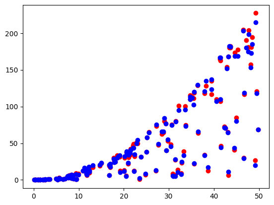

This seems to work relatively well. The average error in the predicted flight distance is 1.9 m which is not too bad, but still larger than I would like!

Polynomial Regression

Polynomial regression is an extension of linear regression that allows for modeling non-linear relationships between the independent and dependent variables. Recall that the input variables are sometime also called “features” when discussing ML. In polynomial regression the output is modeled as a nth degree polynomial: $y = b_0 + b_1 x + b_2 x^2 + \dots + b_n x^n$. The way this is done is very clever, the input features are replaced with new features that are powers of the original. For example, if $x$ is the original feature and $n=3$, then the new features will be $x$, $x^2$, $x^3$. After this transformation the fitting can be done using the same was as linear linear regression. Pretty cool.

Here is Python code that performs the analysis. The accuracy of the results is quite good, with a mean absolute error of 0.092 meters.

from sklearn.preprocessing import PolynomialFeatures
from sklearn.linear_model import LinearRegression

poly = PolynomialFeatures(degree=4, include_bias=False)
X_train_new = poly.fit_transform(X_train)
model = LinearRegression()
model.fit(X_train_new, y_train)
print("model coef =", model.coef_)

X_test_new = poly.fit_transform(X_test)
predictions = model.predict(X_test_new)
print(f"Mean absolute error={mean_absolute_error(y_test, predictions):.3f}")

plt.scatter(X_test[:,1], y_test, c='r')
plt.scatter(X_test[:,1], predictions, c='b')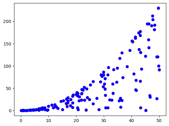

We can also create a 3D scatter plot as follows:

fig = plt.figure()
ax = fig.add_subplot(projection='3d')
ax.scatter(X_test[:,0], X_test[:,1], y_test, c='r')
ax.scatter(X_test[:,0], X_test[:,1], predictions, c='b')
ax.set_xlabel('Angle (deg)')
ax.set_ylabel('Velocity (m/s)')
ax.set_zlabel('Distance (m)')
plt.show()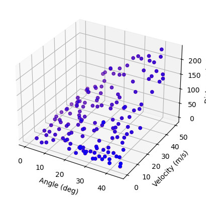

Note 1: Polynomial Regression can be quite accurate and is easy to use. Note that you don’t want to use too high degree polynomials since they tend to be oscillatory.

Note 2: Feature mapping (which is used in Polynomial Regression)  is a very powerful concept that is commonly used ML models.