Neural Network Analysis of Hammer Throw Distance using TensorFlow Keras

Jorgen Bergstrom included in Hammer Throw

2024-05-28 302 words 2 minutes

Contents

Summary

The Keras Sequential model is a simple and straightforward way to build neural networks in Keras, a high-level neural networks API running on top of TensorFlow. The Sequential model allows you to stack layers sequentially, meaning each layer has exactly one input tensor and one output tensor. You start by creating an instance of the Sequential model, then add layers to it one by one. Each layer, such as Dense (fully connected), Convolutional, or LSTM (Long Shor-Term Memory), is added using the add method. The model is compiled with a loss function, an optimizer, and metrics for evaluation using the compile method. Training the model is done using the fit method, which takes the input data and corresponding labels. The Sequential model is particularly useful for building simple feedforward neural networks where layers are added in a linear stack.

Code Location

You can find the code in this example here.

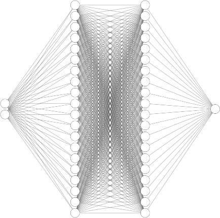
The following Python code implements a Keras NN model that can predict hammer throw distance.

import matplotlib.pyplot as plt
import numpy as np
from sklearn.model_selection import train_test_split
from sklearn.preprocessing import StandardScaler  
from sklearn.metrics import mean_absolute_error 
import keras
from keras import layers

X = np.load('data_X.npy')
Y = np.load('data_Y.npy')
X_train, X_test, y_train, y_test = train_test_split(X, Y, test_size=0.3)

scaler = StandardScaler()
X_train = scaler.fit_transform(X_train)
X_test = scaler.transform(X_test)

model = keras.Sequential()
model.add(keras.Input(shape=(2,)))
model.add(layers.Dense(20, activation='relu', kernel_initializer='he_normal'))
model.add(layers.Dense(20, activation='relu', kernel_initializer='he_normal'))
model.add(layers.Dense(1, activation='linear',  kernel_initializer='he_normal'))
model.compile(optimizer='nadam', loss='mse', metrics=['mean_absolute_error'])
model.fit(X_train, y_train, epochs=10000, batch_size=50, verbose=0)
model.summary()

predictions = model.predict(X_test, verbose=0)
print(f"Mean absolute error={mean_absolute_error(y_test, predictions):.3f}")
plt.scatter(X_test[:,1], y_test, c='r')
plt.scatter(X_test[:,1], predictions, c='b')
plt.xlabel('Velocity (m/s)')
plt.ylabel('Distance (m)')

Here’s the output from running this model:

Total params: 1,506 (5.89 KB)
Trainable params: 501 (1.96 KB)
Non-trainable params: 0 (0.00 B)
Optimizer params: 1,005 (3.93 KB)
Mean absolute error=0.438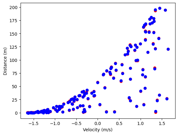

As expected, the predictions from this model are similar to the predictions form the Scikit-Learn NN model.