 Jorgen Bergstrom
Predicting Cancer with a Tiny Autograd Engine
Introduction
In the first two articles of this series we built a reverse-mode autograd engine (engine.py) and a small neural-network library on top of it (nn.py). Together they are about 140 lines of pure Python with no numerical dependencies beyond the standard library.
This article puts them to work on a real problem: predicting whether a breast tumor is malignant from measurements taken from a digitized image. The script is cancer_prediction.py, and it does the whole job with nothing but the Value class and the MLP from the previous articles. We will look at the data, the loss, the training loop, and the cross-validation, and then compare the result against a version of the same problem written in PyTorch, cancer_prediction_torch.py.
The exercise is a good stress test of the engine. If the gradients it computes are wrong anywhere, the network simply will not learn.
The problem and the data
The Breast Cancer Wisconsin dataset ships with scikit-learn and is small enough to run on a laptop:
- 569 samples, 30 numeric features (radius, texture, perimeter, smoothness, …)
- 212 malignant, 357 benign
data = load_breast_cancer()
X = data.data.astype(np.float64)
# sklearn encodes 0 = malignant, 1 = benign; swap that
y = (data.target == 0).astype(np.float64)
One detail matters here. scikit-learn encodes the classes as 0 = malignant and 1 = benign, but the code flips them so that 1 is the malignant, positive class. That is the convention the rest of the script assumes when it computes probabilities and losses. It is an easy thing to get backwards, and getting it backwards silently inverts every interpretation of the output.
The features live on wildly different scales (a radius and a smoothness are not comparable numbers), so they are standardised. We will come back to where that happens, because doing it in the wrong place leaks information across the cross-validation folds.
Binary cross-entropy with logits
The network produces a single real number per sample — a logit z. The probability of malignancy is sigmoid(z), and the loss is binary cross-entropy:
$$\mathcal{L} = \frac{1}{n}\sum_{i=1}^{n}\Big[\underbrace{\log\big(1 + e^{z_i}\big)}_{\text{softplus}(z_i)} - y_i z_i\Big].$$
This is algebraically the same as the more familiar form
$$-\big[y\log p + (1-y)\log(1-p)\big], \qquad p = \text{sigmoid}(z),$$
but it never takes the logarithm of a probability that has saturated to 0 or 1. That is why every serious framework offers a “with logits” loss: the loss expects the raw logit and applies the sigmoid internally in a numerically stable way.
In nn.py we deliberately made the final layer linear, so the model already returns a logit. The scratch version builds the softplus branch by hand:
def bce_with_logits_loss(model, X, y):
    losses = []
    for xi, yi in zip(X, y):
        z = model([Value(v) for v in xi])

        if z.data > 0:
            # log(1 + e^z) = z + log(1 + e^-z)  (exponent stays <= 0)
            softplus = z + (1.0 + (-z).exp()).log()
        else:
            # log(1 + e^z)  (exponent stays <= 0)
            softplus = (1.0 + z.exp()).log()

        # softplus(z) - y*z  ==  BCE(sigmoid(z), y)
        losses.append(softplus - yi * z)

    return sum(losses) * (1.0 / len(losses))
The branch is the stability trick. For a large positive z, computing log(1 + e^z) directly would overflow e^z; rewriting it as z + log(1 + e^{-z}) keeps the exponent non-positive. For a non-positive z the direct form is already safe. Either way the argument of log is at least 1, so the result is finite.
Notice how the loop reads: wrap each feature in a Value, call the model to get a Value logit, and build the softplus term from exp, log, negation, and multiplication. Every one of those is an operation the engine already knows how to differentiate. There is no separate loss gradient to derive or code — calling .backward() on the averaged loss differentiates the entire expression, network included.
For validation we want a plain number rather than another graph, so there is a separate helper that works on the predicted probabilities directly and clips them away from 0 and 1.
The model and the training loop
The model is the MLP from the previous article, with two hidden layers of 16 units and a single linear output:
model = MLP(X.shape[1], HIDDEN) # HIDDEN = [16, 16, 1]Training is mini-batch SGD with a learning rate that decays linearly from LR to one tenth of LR over the run. The core of the loop should look familiar from the nn.py article:
for epoch in range(EPOCHS):
    # learning rate decays linearly to 10% of its initial value
    lr = LR * (1.0 - 0.9 * epoch / max(1, EPOCHS - 1))
    perm = rng.permutation(n)
    epoch_loss = 0.0

    for s in range(0, n, BATCH_SIZE):
        idx = perm[s:s + BATCH_SIZE]
        data_loss = bce_with_logits_loss(model, X_tr[idx], y_tr[idx])
        total_loss = data_loss + l2_regularization(model, ALPHA)

        model.zero_grad()
        total_loss.backward()
        for p in model.parameters():
            p.data -= lr * p.grad

        epoch_loss += data_loss.data * len(idx)

    history["train_loss"].append(epoch_loss / n)
    history["val_loss"].append(
        bce_from_probs(y_va, predict_proba(model, X_va)))
Three things are worth pointing out:
model.zero_grad()beforebackward(). The backward pass accumulates into.grad, so gradients must be cleared each step. This is exactly the caveat from the engine article, and exactly whatzero_grad()is for.- The update is one line.
p.data -= lr * p.gradis vanilla gradient descent; there is no optimizer object and no hidden state. Every parameter is just a Python float living inside aValue. - Momentum and weight decay are absent. The only regularisation is an explicit L2 penalty,
alpha * sum((p * p for p in model.parameters())), added to the data loss. It is weak (alpha = 1e-4), which we will see in the results.
Cross-validation without leaking data
A single train/validation split can be lucky or unlucky, so the script uses stratified k-fold cross-validation: the data is split into five folds that preserve the malignant/benign ratio, and each fold serves as the validation set exactly once.
The subtle part is the feature scaling:
for fold, (tr, va) in enumerate(splitter.split(X, y), start=1):
    scaler = StandardScaler()
    X_tr = scaler.fit_transform(X[tr])
    X_va = scaler.transform(X[va])

    model = MLP(X.shape[1], HIDDEN)
    history = train(model, X_tr, y[tr], X_va, y[va])
    ...
The scaler is fit only on the training fold and then applied to the validation fold. If we standardised the whole dataset before splitting, the training folds would have seen the mean and standard deviation of the validation samples — a small but real case of data leakage that makes the reported accuracy look better than it is. Fitting inside the loop is the honest way to do it, and it is the reason the model is rebuilt from scratch on every fold.
Results
Running cancer_prediction.py gives:
dataset: 569 samples, 30 features
classes: 212 malignant, 357 benign
fold 1/5: train loss 0.0406, val loss 0.2677, acc 96.49%
fold 2/5: train loss 0.0260, val loss 0.2089, acc 92.98%
fold 3/5: train loss 0.0447, val loss 0.0476, acc 98.25%
fold 4/5: train loss 0.0549, val loss 0.0999, acc 95.61%
fold 5/5: train loss 0.0553, val loss 0.1547, acc 93.81%
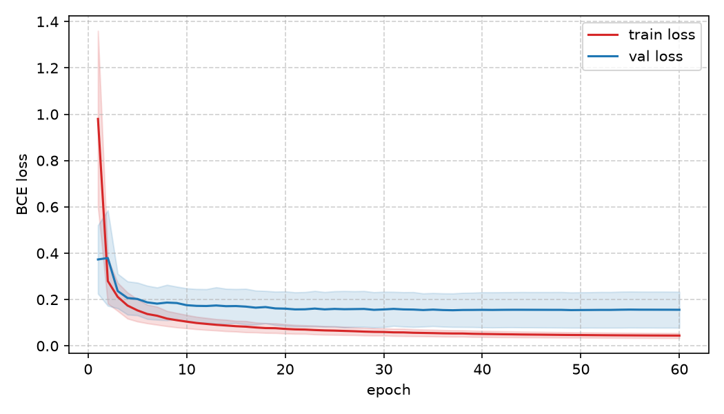
That is a mean validation accuracy of 95.4% ± 1.9% across the five folds. The validation loss varies a lot fold to fold (from 0.048 to 0.268) while the training loss stays around 0.04, which is the classic signature of mild overfitting: with alpha = 1e-4 the L2 penalty is not holding the weights back much, and with only 785 parameters and ~455 training samples per fold there is room to memorise.
Still, the important result is not the accuracy number. It is that a neural network trained entirely by an autograd engine written from scratch in 80 lines reaches the same ballpark as a conventional implementation. The gradients are correct.
The script also saves a training-curve figure, cancer_training.png, showing the mean and standard deviation of the train and validation losses across the folds:
The same problem in PyTorch
Seeing the same problem solved in a framework is useful, both as a sanity check on the from-scratch result and to see what the framework buys us. cancer_prediction_torch.py is the vectorised counterpart: same dataset, same architecture, same folds, same hyperparameters.
The differences fall into four categories.
The model is a module rather than a hand-built graph.
class MLP(nn.Module):
    def __init__(self, nin, nouts):
        super().__init__()
        sizes = [nin] + nouts
        layers = []
        for i in range(len(nouts)):
            layers.append(nn.Linear(sizes[i], sizes[i + 1]))
            if i != len(nouts) - 1:
                layers.append(nn.ReLU())
        self.net = nn.Sequential(*layers)

    def forward(self, x):
        return self.net(x)
The loss comes from the library, and it is the same stable form we wrote by hand:
def bce_with_logits_loss(model, X, y):
    logits = model(X).squeeze(-1)
    return F.binary_cross_entropy_with_logits(logits, y)
There is an optimizer object, so the update loop disappears:
optimizer = torch.optim.SGD(model.parameters(), lr=LR)
...
optimizer.zero_grad()
total_loss.backward()
optimizer.step()  # p.data -= lr * p.grad
The code opts into the GPU with two lines. Every tensor and the model are placed on DEVICE, which is CUDA when available and CPU otherwise:
DEVICE = "cuda" if torch.cuda.is_available() else "cpu"

model = MLP(X.shape[1], HIDDEN).to(DEVICE)                 # move the parameters
X_tr = torch.as_tensor(X_tr, dtype=torch.float32, device=DEVICE)  # move the data
On the machine this ran on, that line reported:
device: cuda (NVIDIA GeForce RTX 5060 Ti)and the results were:
fold 1/5: train loss 0.0542, val loss 0.0709, acc 97.37%
fold 2/5: train loss 0.0526, val loss 0.0842, acc 98.25%
fold 3/5: train loss 0.0626, val loss 0.0289, acc 99.12%
fold 4/5: train loss 0.0460, val loss 0.0881, acc 96.49%
fold 5/5: train loss 0.0520, val loss 0.0975, acc 96.46%
a mean validation accuracy of 97.5% ± 1.0%, with training running in well under a second per fold.
Comparing the two
cancer_prediction.py | cancer_prediction_torch.py | |
|---|---|---|
| Backend | Value scalars | PyTorch tensors |
| Gradients | our 80-line engine | torch.autograd |
| Update | manual p.data -= lr * p.grad | optimizer.step() |
| Batch handling | a Python loop over samples | vectorised over the batch |
| Device | CPU (single-threaded Python) | CUDA or CPU |
| Mean accuracy | 95.4% ± 1.9% | 97.5% ± 1.0% |
The PyTorch version is faster and scores a little higher, but it is worth being careful about what that does and does not show:
- The speed-up is mostly vectorisation, not the GPU. The framework replaces the per-sample Python loop with a handful of array operations, and that is the dominant win. For a model this small, kernel-launch and host/device transfer overhead are comparable to the compute; the GPU is not the interesting part. (The torch file says as much in its own teaching note.)
- The accuracy gap is not a fair fight. The two scripts initialise weights differently, shuffle in a different order, and the CUDA results are not bit-identical to CPU even with the same seed. A single percentage point over five folds is well within that noise. The honest conclusion is that both are in the same range, not that one is better.
- The from-scratch version is not meant to compete. Its value is that every gradient, every update, and every loss term is visible and derived from the same small set of rules. The PyTorch version is what you would actually ship.
Two things to keep in mind
- The loss wants logits, not probabilities. Because the final layer is linear, the model returns a raw logit and
binary_cross_entropy_with_logits(or our hand-built softplus branch) consumes it directly. Applying a sigmoid to the output before the loss would undo the stability trick and flatten the gradients when the prediction is confidently wrong — precisely when we need them most. - Scale inside the fold. Feature standardisation must be fit on the training split only. Doing it once over the whole dataset is easy to write and easy to miss, and it inflates cross-validation scores by leaking information from the validation samples.
Wrapping up the series
Across three files — engine.py, nn.py, and cancer_prediction.py — we went from “what is a derivative of a scalar” to a working, cross-validated classifier with no machine-learning dependencies. The PyTorch companion shows the same problem in the idiom most people actually use, and the two agree to within noise. The point of the exercise was never to replace PyTorch; it was to make the machinery under it something you can read in one sitting.