 Jorgen Bergstrom
Backpropagation Part 3: 1 Hidden Layer, N Perceptrons
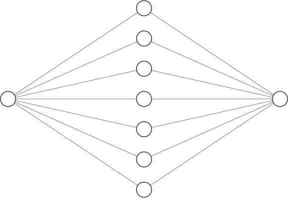
[1 Input] + [1 Hidden Layer with N Perceptrons] + [1 Output]
In this example I will extend my previous code to be able to handle a hidden layer with N perceptrons. As before, I will demonstrate the use of the neural network by fitting it to the following mathematical function: $y = 0.1 + 0.1 \cdot x^2$ over the range $x \in [0, 10]$. The C++ implementation for this example can be found in my github account. The code supports the following features: different activation functions, different initiation functions, and different optimization methods.
The C++ code for the main function is listed here:
// 2 Layers: 1 input, N hidden, 1 output
#include <iostream>
#include <vector>
#include <cassert>
#include "Neural_Network_1N1.h"

int
main(int argc, char *argv[])
{
    std::cout << "Generate training data" << std::endl;
    constexpr int N {100};  // number of training features
    std::vector<double> x(N), y(N);
    for (int f=0; f < N; f++) {
        x[f] = 10.0 * f / N;
        y[f] = 0.1 * (1.0 + x[f]*x[f]);
    }

    // normalize training data
    std::cout << "Normalize the training data" << std::endl;
    double minX, maxX, minY, maxY;
    minX = maxX = x[0];
    minY = maxY = y[0];
    for (int i=0; i < N; i++) {
        minX = std::min(minX, x[i]);
        maxX = std::max(maxX, x[i]);
        minY = std::min(minY, y[i]);
        maxY = std::max(maxY, y[i]);
    }
    for (int i=0; i < N; i++) {
        x[i] = (x[i] - minX) / (maxX - minX);
        y[i] = (y[i] - minY) / (maxY - minY);
    }

    //---------------------------------------------------
    std::cout << "Initialize the NN" << std::endl;
    Neural_Network_1N1 nn;
    int nrHidden {8};
    nn.init(nrHidden, 1, ActivationType::ReLU, ActivationType::linear); // number of perceptrons in hidden layer

    //---------------------------------------------------
    Neural_Network_Settings settings;
    int method {0};
    if (argc==2) {
        method = atoi(argv[1]);
    } else {
        std::cout << "What method do you want to use to fit the NN [1=vanilla, 2=non-linear optimization, 3=Adam]: ";
        std::cin >> method;
    }

    switch (method) {
        case 1: // mini-batch gradient descent with constant learning rate
            settings.method = 1;
            settings.batch_size = 10;
            settings.max_epochs = 10000;
            settings.ftol_abs = 1e-5;
            settings.learning_rate = 1.0e-3;
            settings.clipval = 100;
            settings.verb = 0;
            break;
        case 2: // non-linear optimization (LN_SBPLX)
            settings.method = 2;
            settings.maxeval = 40000;
            settings.batch_size = x.size();
            settings.ftol_rel = 0;
            settings.ftol_abs = 0;
            settings.xtol_rel = 0;
            settings.verb = 1;
            break;
        case 3: // mini-batch gradient descent with Adam optimizer
            settings.method = 3;
            settings.batch_size = 10;
            settings.max_epochs = 10000;
            settings.alpha = 0.001;
            settings.beta1 = 0.9;
            settings.beta2 = 0.999;
            settings.epsilon = 1.0e-8;
            settings.ftol_abs = 1e-6;
            settings.clipval = 100;
            settings.verb = 0;
            break;
        default:
            assert(false);
    }

    //---------------------------------------------------
    std::cout << "Fit the neural network" << std::endl;
    nn.fit(x, y, settings);
    std::cout << "\nFinal Results:" << std::endl;
    std::cout << "   number of epochs = " << nn.err.size() << std::endl;
    std::cout << "   number of function evaluations = " << nn.nrFuncEvals.back() << std::endl;
    std::cout << "   error = " << nn.err.back() << std::endl;
    nn.print_vec("   params", nn.params);
    nn.print_err_to_file("NN_err.txt");
    nn.save_predictions_to_file(x, "NN_results.txt");
    std::cout << "done." << std::endl;
}
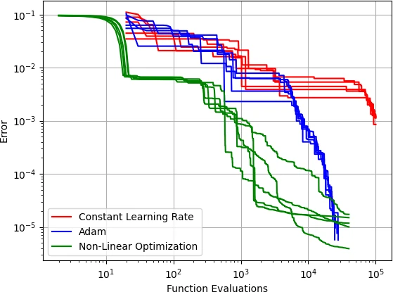
The figure below compares the performance of different optimization methods when training our model. We can see that the Adam optimizer outperforms a constant learning rate. However, the nonlinear optimization method SBPLX converges even more rapidly. SBPLX is a derivative-free optimization algorithm that is based on the Nelder-Mead simplex method. It’s important to note that while SBPLX may require fewer iterations to converge, each iteration can be computationally expensive. For most machine learning tasks, the gradient descent method with the Adam optimizer is the recommended approach due to its balance of speed and efficiency.