Backpropagation Part 2: 1 Hidden Layer, 2 Perceptrons

Jorgen Bergstrom included in Neural Networks

2024-10-22 818 words 4 minutes

Contents

[1 Input] + [1 Hidden Layer with 2 Perceptrons] + [1 Output]

In this example I will create a simple neural network that has one input, one hidden layer with 2 perceptrons, and one output. I will then fit that neural network to the following mathematical function: $y = 0.1 + 0.1 \cdot x^2$ over the range $x \in [0,10]$.

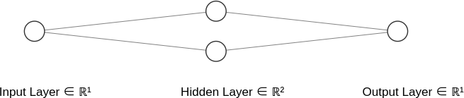
C++ code to solve this problem is listed below:

// 2 Layers: 1 input, 2 hidden, 1 output
#include <iostream>
#include <fstream>
#include <algorithm>
#include <cassert>
#include <vector>
#include <cmath>
#include <random>

double
activation(double x, int type)
{
    if (type==1) return std::max(0.0, x); // ReLU
    if (type==2) return 1.0 / (1.0 + exp(-x)); // sigmoid
    if (type==3) return x; // linear
    return 0;
}

double
activation_der(double x, int type)
{
    if (type==1) return (x < 0)? 0 : 1; // ReLU
    if (type==2) return activation(x,type) * (1.0 - activation(x,type)); // sigmoid
    if (type==3) return 1; // linear
    return 0;
}

int
main(int argc, char *argv[])
{
    constexpr int atype {1};
    std::cout << "Generate training data" << std::endl;
    constexpr int N {100};
    std::vector<double> x(N), target(N);
    for (int i=0; i < N; i++) {
        x[i] = 10.0 * i / N;
        target[i] = 0.1 * (1.0 + x[i]*x[i]);
    }
    std::cout << "Initialize parameters" << std::endl;
    double w11, w12, w21, w22, b11, b12, b2;
    w11 = 0.75;
    b11 = -1.0;
    w12 = 1;
    b12 = -6;
    w21 = 1;
    w22 = 1;
    b2 = 0;
    double eta {1.0e-4}; // learning rate

    std::cout << "Backpropagation" << std::endl;
    constexpr int max_epochs {10000};
    std::vector<double> err(max_epochs);
    double dw11_sum, dw12_sum, dw21_sum, dw22_sum, db11_sum, db12_sum, db2_sum;
    double err2_sum;

    for (int epoch=0; epoch < max_epochs; epoch++) {
        std::cout << "  epoch=" << epoch << std::endl;
        if (true) { // Vanilla Backpropagation: loop through all training data
            dw11_sum = dw12_sum = dw21_sum = dw22_sum = db11_sum = db12_sum = db2_sum = 0;
            err2_sum = 0;
            for (int i=0; i < N; i++) {
                double x11 = activation(w11 * x[i] + b11, atype);
                double x12 = activation(w12 * x[i] + b12, atype);
                double y   = activation(w21 * x11 + w22 * x12 + b2, atype);
                double tmp = eta * (target[i] - y);
                // L2
                double tmp2 = tmp * activation_der(w21 * x11 + w22 * x12 + b2, atype);
                dw21_sum += tmp2 * x11;
                dw22_sum += tmp2 * x12;
                db2_sum   += tmp2;
                // L1-1
                double tmp1 = tmp2 * activation_der(w11 * x[i] + b11, atype);
                dw11_sum += tmp1 * x[i];
                db11_sum += tmp1;
                // L1-2
                tmp1 = tmp2 * activation_der(w12 * x[i] + b12, atype);
                dw12_sum += tmp1 * x[i];
                db12_sum += tmp1;
                err2_sum += pow(target[i] - y, 2.0);
            }
            w11 += dw11_sum / N;
            w12 += dw12_sum / N;
            w21 += dw21_sum / N;
            w22 += dw22_sum / N;
            b11 += db11_sum / N;
            b12 += db12_sum / N;
            b2  += db2_sum  / N;
            err[epoch] = 0.5 * err2_sum/N;
        }
        std::cout << "    err2 = " << err[epoch] << std::endl;
    }

    std::cout << "Final parameters" << std::endl;
    std::cout << "  w11 = " << w11 << std::endl;
    std::cout << "  b11 = " << b11 << std::endl;
    std::cout << "  w12 = " << w12 << std::endl;
    std::cout << "  b12 = " << b12 << std::endl;
    std::cout << "  w21 = " << w21 << std::endl;
    std::cout << "  w22 = " << w22 << std::endl;
    std::cout << "  b2  = " << b2 << std::endl;
    std::cout << std::endl;
    std::cout << "Model Predictions" << std::endl;
    std::ofstream eFile("NN_err.txt");
    assert(eFile.is_open());

    for (int i=0; i < err.size(); i++) {
        eFile << err[i] << std::endl;
    }
    eFile.close();
    std::ofstream oFile("NN_results.txt");
    assert(oFile.is_open());
    for (int i=0; i < N; i++) {
        double x11 = activation(w11 * x[i] + b11, atype);
        double x12 = activation(w12 * x[i] + b12, atype);
        double y   = activation(w21 * x11 + w22 * x12 + b2, atype);
        oFile << x[i] << ", " << target[i] << ", " << y << std::endl;
    }
    oFile.close();
    std::cout << "done." << std::endl;
}

The results from running this code is plotted in the following figure.

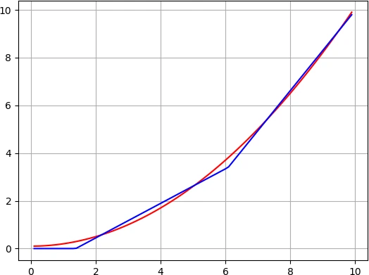
As expected, having 2 perceptrons in the hidden layer allows the neural network more accurately predict the response compared to just having 1 perceptron (see this example).

This problem can also be solved using the Keras Python library. Note that the Python code runs significantly slower than the C++ code listed above.

import matplotlib.pyplot as plt
import numpy as np
import keras
from keras import layers

print("\n\n")
print("generate training data")
N = 100
x = np.empty(N)
target = np.empty(N)
for i in range(N):
    x[i] = 10 * i / N
    target[i] = 0.1 * (1.0 + x[i]**2)

print("create model")
model = keras.Sequential()
model.add(keras.Input(shape=(1,)))
model.add(layers.Dense(2, activation='relu', kernel_initializer='he_normal'))
model.add(layers.Dense(1, activation='relu', kernel_initializer='he_normal'))
model.compile(optimizer='nadam', loss='mse', metrics=['mean_absolute_error'])

print("fit model")
model.fit(x, target, epochs=1000, verbose=1)
model.summary()

print("compare predictions to target")
predictions = model.predict(x, verbose=0)
model.summary()

print("L1 weights: ", model.layers[0].get_weights())
print("L2 weights: ", model.layers[1].get_weights())
print("plot results")
plt.plot(x, target, 'r-')
plt.plot(x, predictions, 'b-')
plt.grid()
plt.savefig('plot_predictions_keras.png')
plt.show()