Backpropagation Part 1: Single Perceptron

Jorgen Bergstrom included in Neural Networks

2024-10-20 1063 words 5 minutes

Contents

One Network Layer with 1 Input and 1 Output

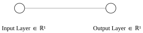
The simplest neural network architecture consists of a single perceptron. This network has only one input and one output, making it a highly streamlined model. While suitable for theoretical understanding, it is insufficient for real-world applications due to its limited capacity. However, it serves as a fundamental building block for studying the principles of backpropagation and training neural networks.

Code Location

You can find the source code for this example here.

What is a Perceptron?

A perceptron is a simplified model of a neuron that can learn to classify data by linearly separating the input data into different categories. It is a fundamental building block of artificial neural networks and plays a role in machine learning algorithms like linear regression and classification.

Structure of a Perceptron:

Input layer: Receives the raw data.
Weighting layer: Multiplies the input data by weight values.
Bias term: Adds a constant value to the weighted input.
Activation function: Determines whether the output is positive or negative.
Output layer: Produces the final classification or prediction.

How it works:

The input data is multiplied by the weight values.
The bias term is added to the weighted input.
The activation function is applied to the sum, which determines the output.
The output is either positive or negative, indicating the classification or prediction.

Learning process:

The perceptron learns by adjusting the weight values and bias term.
It compares the predicted output with the actual output.
Errors are corrected by adjusting the weights and biases in the direction that reduces the error.

The following pseudocode explains how we can analyze this simple neural network (NN):

Input: x
Output: y = f(w * x + b)
Desired result (target): d
# The scalar function f(.) is called the activation funciton
# f'(.) is the derivative of the activation function
# The goal is to minimize the error: 
e = 0.5 * (d - y)^2
# That is, find the parameters [w,b] that minimize the error e
# We can do that by taking a small step in the negative gradient direction
# Gradient Descent approach (where eta=learning rate):
dw = -eta * de/dw
db = -eta * de/db
# The new weights therefore become:
# (where eta is small constant called the learning rate)
w += -eta * de/dw
b += -eta * de/db
# In this case (using the chain rule):
de/dw = (d-y) * (-1) * dy/dw
      = (d-y) * (-1) * f’(w*x+b) * x
de/db = (d-y) * (-1) * f’(w*x+b)
# In summary:
w_new = w_old + eta * (d-y) * f’(w*x+b) * x
b_new = b_old + eta * (d-y) * f’(w*x+b)

The algorithm to find [w,b] therefore becomes:

w = random number
b = random number
eta = small number
for epoch in range(100):
    tmp1 = w*x+b
    y = f(tmp1)
    tmp2 = eta * (d-y) * f’(tmp1)
    w = w + tmp2 * x
    b = b + tmp2

Activation Functions

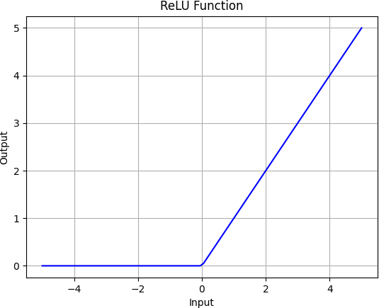
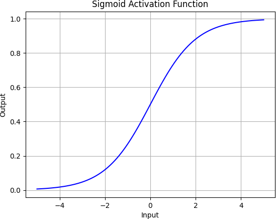
There are many different activation functions that can be used. Here are some examples (in C++ code format). The perhaps two most commonly used activation functions are ReLU and sigmoid. The ReLU activation is often used for classification tasks with linearly separable data, and sigmoid activatation is often used for logistic regression and binary classification.

double
Neural_Network_1N1::activation(double x, ActivationType type)
{
    switch (type) {
        case ActivationType::ReLU:
            return std::max(0.0, x);
        case ActivationType::sigmoid:
            return 1.0 / (1.0 + exp(-x));
        case ActivationType::linear:
            return x;
        case ActivationType::Leaky_ReLU:
            return std::max(0.1*x, x);
        default:
            throw std::runtime_error("Unsupported activation type");
    }
}

double
Neural_Network_1N1::activation_der(double x, ActivationType type)
{
    switch (type) {
        case ActivationType::ReLU:
            return (x < 0)? 0 : 1;
        case ActivationType::sigmoid:
            return activation(x,type) * (1.0 - activation(x,type));
        case ActivationType::linear:
            return 1;
        case ActivationType::Leaky_ReLU:
            if (x < 0) return 0.1;
            return 1;
        default:
            throw std::runtime_error("Unsupported activation type");
    }
}

Complete Example

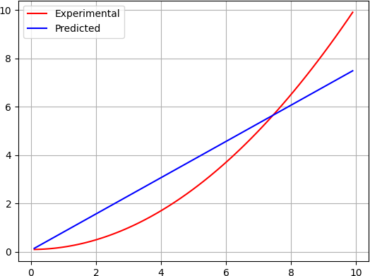
In this example I will try to fit a single layer, single perceptron network model to a non-linear mathematical function: $y = 0.1 + 0.1 \cdot x^2$.

Here’s the C++ code.

#include <iostream>
#include <fstream>
#include <algorithm>
#include <cassert>
#include <vector>
#include <cmath>

double
ReLU(double x) {
    return std::max(0.0, x);
}

double
ReLU_der(double x) {
    if (x < 0) return 0;
    return 1;
}

int
main(int argc, char *argv[])
{
    std::cout << "Generate training data" << std::endl;
    constexpr int N {100};
    std::vector<double> x(N), target(N);
    for (int i=0; i < N; i++) {
        x[i] = 10.0 * i / N;
        target[i] = 0.1 * (1.0 + x[i]*x[i]);
    }
    std::cout << "Initialize parameters" << std::endl;
    double w {0.1};
    double b {0.1};
    double eta {1.0e-4}; // learning rate
    std::cout << "Backpropagation" << std::endl;
    constexpr int max_epochs {3000};
    std::vector<double> err(max_epochs);
    for (int epoch=0; epoch < max_epochs; epoch++) {
        std::cout << "  epoch=" << epoch << std::endl;
        double dw_sum {0};
        double db_sum {0};
        double err2_sum {0};
        for (int i=0; i < N; i++) {
            double tmp1 = w * x[i] + b;
            double y = ReLU(tmp1);
            double tmp2 = eta * (target[i] - y) * ReLU_der(tmp1);
            dw_sum += tmp2 * x[i];
            db_sum += tmp2;
            err2_sum += pow(target[i] - y, 2.0);
        }
        w += dw_sum / N;
        b += db_sum / N;
        double e = 0.5 * err2_sum/N;
        if (epoch == 0) {
            err[0] = e;
        } else {
            err[epoch] = std::min(err[epoch-1], e);
        }
        std::cout << "    w = " << w << std::endl;
        std::cout << "    b = " << b << std::endl;
        std::cout << "    err2 = " << err[epoch] << std::endl;
    }

    std::cout << "Model Predictions" << std::endl;
    std::ofstream eFile("NN_err.txt");
    assert(eFile.is_open());

    for (int i=0; i < err.size(); i++) eFile << err[i] << std::endl;
    eFile.close();
    std::ofstream oFile("NN_results.txt");
    assert(oFile.is_open());

    for (int i=0; i < N; i++) {
        double y = ReLU(w * x[i] + b);
        oFile << x[i] << "\t" << target[i] << "\t" << y << std::endl;
    }
    oFile.close();
}

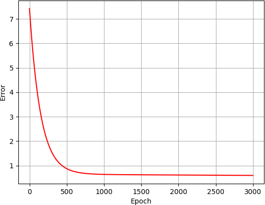
The results from running this code is plotted in the following 2 figures. The red line in the figure to the left is the target function. Since the ReLU function is bilinear, the predicted blue curve clearly cannot match the shape of the target function. The figure to the right shows that the error converges towards the minimum possible value. The rate of convergence, however, is not very good as it takes more than 1,000 function evaluations to reach the target value. Switching to a different optimizer (like the Adam method) would help. That will be covered in a later article.